Back in November of 1969 a young Don Knuth gave his first lecture as a Stanford professor. The lecture was on a new field in Computer Science called Analysis of Algorithms, a field that Knuth invented and named. Recently, Knuth recreated that lecture so that it could be filmed for a university series of videos on important topics. The video is really excellent and everyone in our field should spend the hour to watch it.
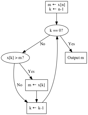
Because the Analysis of Algorithms field was new and mostly unknown, Knuth spent the lecture on an example of analyzing an algorithm. He choose a very simple problem. Given a sequence of numbers \(x_1, x_{2},\ldots,x_n\), find the maximum number, \(m\), in the sequence. We can assume the the \(x_i\) are unique and that every ordering is equally likely. To solve the problem, Knuth chose the obvious algorithm captured by the flow chart below.

At first glance, it’s hard to see what there is to analyze. The algorithm requires an array of size \(n\) and the two additional variables \(m\) and \(k\) for a total of \(n+2\) so it requires \(O(n)\) space. Similarly, it’s easy to see that we go through the loop \(n-1\) times before we terminate so its time is \(O(n)\) too.
In fact, with one exception it’s trivially easy to specify how many times each node in the flow chart is executed. The k == 0? test is made \(n\) times and the x[k] > m test is made \(n-1\) times for example. The one exception is the m ← x[k] box. It is executed only when a new maximum is found. Call the number of times it’s executed \(A\). What can we say about it?
Obviously, \(A=0\) when the maximum number is last in the sequence and it’s \(n-1\) when \(x_1 > x_2 > \ldots >x_n\) but what is its average (or expected) value? If you don’t think about it too hard, \(n/2\) seems like a good guess.
It’s easy to calculate the \(n=3\) case and when you do, you find that the average value of \(A\) is \(5/6\) so our \(n/2\) guess is incorrect. Most of the lecture is spent finding the correct answer, which turns out to be \(H_{n}-1\) where \(H_n\) is the \(n\)th partial sum of the harmonic series. Therefore, \(A \approx \ln(n)\) and the average value of \(A\) for \(n=1,000,000\) is about 13.5; much different from what you might have expected.
Knuth says that the techniques he uses in this analysis appear over and over again so the simple problem turns out to be an important and instructive example. If you’d like to explore the analysis at your own pace, you can find the same example in Section 1.2.10 of AOCP.
